2/5/2022: Spreadsheet to Track Time Used for Each Party and for Each Examination
The Tip of the Night for September 4, 2021 discussed how to use the SUMIF formula in Excel to set up a spreadsheet to track the time each party uses in a trial. Tonight I have posted a spreadsheet which you can use to track the time used by each party on each day with the SUMIFS formula, and the time that each witness examination takes using the SUMIF formula.
Begin by entering the date, witness examination description, party name, attorney name, start time, and end time in columns A to F. In column B, ‘Witness’ enter not only unique descriptions for each direct and cross examination, but also enter notes for lunch and time spent by the parties discussing procedural matters with the court. Be sure to enter a description for each examination or other event consistently with the same exact characters. In column C enter the name of the party conducting each examination, opening or closing, and also consistently enter notes for court and break time .

A simple subtraction formula in column G will calculate the amount of time used for each entry. Be sure to format this column for as h:mm:ss in the Custom setting.
Columns L to Q will track the cumulative time used by each party and the court (and used for breaks) by utilizing the SUMIFS formula. This formula works by searching for the values to be added up in first referenced column; then searching for a value given the second referenced column [this is case it looks for the date in L2 given in column A], and then only adding the values given at the end of formula listed in the third referenced column [so it looks for the party name given in M1 in column C].
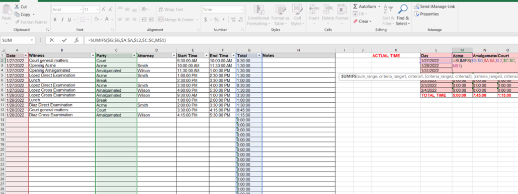
The SUMIFS formula looks for two criteria in different columns and then only adds up the value given in a third column when the given values are matched in the other two columns. You want to use an absolute reference with dollar signs so the same column for the date is always referenced by pulling the formula to the right, and the same row is used for the party name, and then double dollar signs so each column which is searched for a value so it stays the same as the formula is pulled to the right.
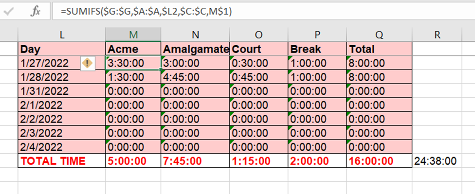
The last row in this array uses a simple SUM formula to add up the time used by each party.
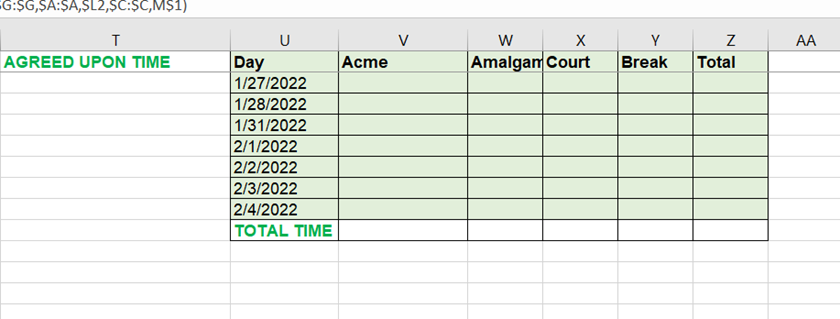
Columns U to Z are simply used to track the amount of time used that the parties agreed to. Manual entries should be made in each cell. It certainly seems as though each side always disagrees on exactly how much time they have taken up.
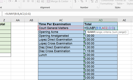
In column AC enter just once each description for an examination or other event used in column C. The SUMIF formula in column AD will then searcy for these values in column B and in the rows where the value is found add up the time in column G.
2/21/2022: Negative Lookahead Regular Expression Search
In order to run a negative lookahead regular expression search, you can enclose the string you do NOT want the searched for string to appear in front of, in parentheses with a question mark and exclamation point before the given string. So in this example this search: Albany(?!\s+NY)
. . . will find any instance in which Albany is not followed by ‘ NY’.
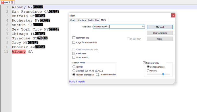
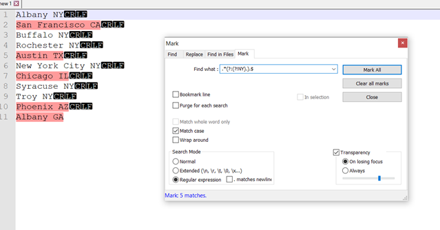
This search can be modified to find any string – .* – which does not precede the state abbreviation NY – (?:(?!NY).).$
.*(?:(?!NY).).$
2/18/2022: Making Multiple Selections from an Excel Drop Down List
It’s widely known that Excel’s Data Validation tool can be used to create a drop down list for all cells in a selected range. You’ll simply be able to click on an down arrow next to a cell and select the entry. This feature can speed up a lengthy manual review of documentation tracked on a spreadsheet. Tonight’s tip will show how you can use VBA code to change this tool to allow for multiple entries from the list to be saved in a cell.
To get started follow these steps:
1. Select the data range you want the ‘pick list’ to be available for.
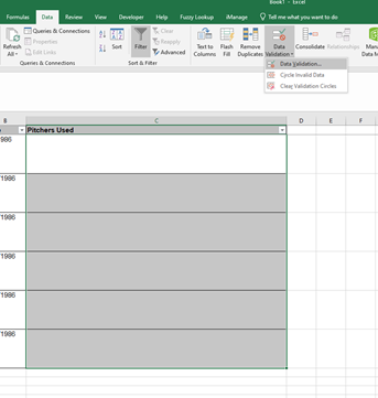
2. Go to Data . . . Data Validation
3. In the dialog box on the Settings tab, choose ‘List’ from the Allow menu. Then click on the arrow next to the Source box to select the data range which will contain the entries you want to appear in the drop down list. The entries can be listed on a different worksheet.
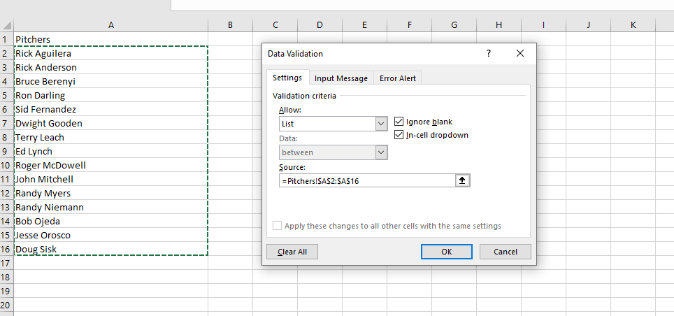
If you have to add more items to the list as you go along, check off the box labeled, ‘Apply these changes to all other cells with the same settings’, and then expand the source range.
4. This will give you a drop down list that will let you select any one of the entries for the cell. If you select a second entry, the first entry will be overwritten.
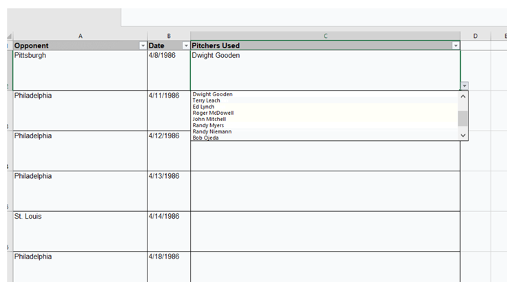
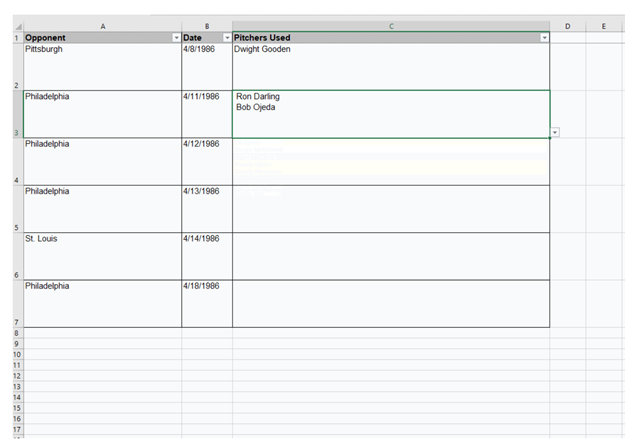
You can use VBA code posted here, and modified below to make it possible to select multiple entries. The modified version lets you clear the cell after entries have been made (thanks to Susan Lynn for her suggestion); leaves the first entry you select at the beginning of the cell; and puts each new entry on a new line.
On this line of the VBA code you can set the delimiter you want to use between the entries.
xStrNew = ” ” & Target.Value & Chr(10)
In my version of the code I’ve entered the Chr(10) reference to put each new entry on a separate line. If ‘Chr(10)’ is changed to “; “ each new entry will be separated with a semi-colon.
In order to clear a cell, select it and choose ‘Clear Contents’ from the right click menu.
Private Sub Worksheet_Change(ByVal Target As Range)
‘UpdatebyExtendoffice20180510
Dim I As Integer
Dim xRgVal As Range
Dim xStrNew As String
Dim xStrOld As String
Dim xFlag As Boolean
Dim xArr
On Error Resume Next
Set xRgVal = Cells.SpecialCells(xlCellTypeAllValidation)
If (Target.Count > 1) Or (xRgVal Is Nothing) Then Exit Sub
If Intersect(Target, xRgVal) Is Nothing Then Exit Sub
Application.EnableEvents = False
xFlag = True
xStrNew = ” ” & Target.Value & Chr(10)
Application.Undo
xStrOld = Target.Value
If InStr(1, xStrOld, xStrNew) = 0 Then
xStrNew = xStrOld & xStrNew
Else
xStrNew = “”
End If
Target.Value = xStrNew
Application.EnableEvents = True
End Sub
2/25/2022: Javascript to change annotation types in Acrobat
Using javascript posted here by Evermap, and copied below you can automatically transform annotations from one type in Adobe Acrobat to another type. It will not only allow you to convert highlights, underlined text, and crossed out text, but also to change from proposed redactions to any one of these annotations – but not vice versa.
In order to add the script to a new action in Acrobat, select the Action Wizard tool and then click on ‘New Action’, and choose ‘Execute JavaScript’ from the ‘More Tools’ drop down menu.
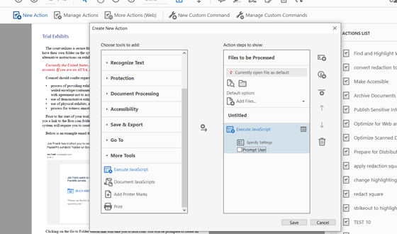
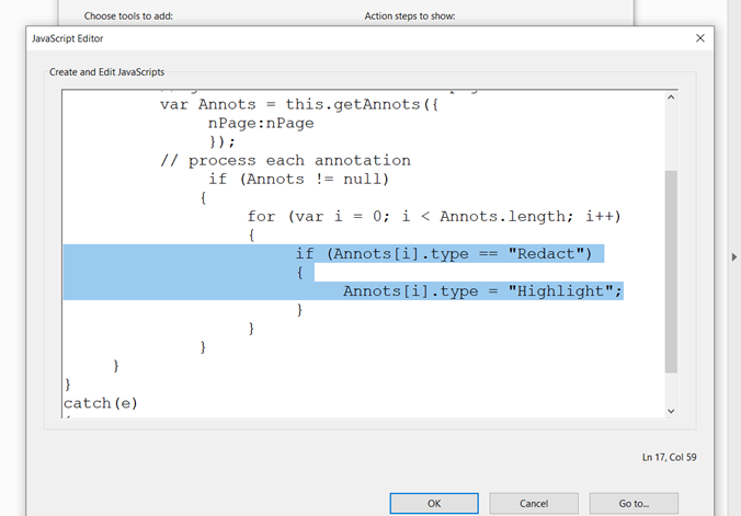
Click on ‘Specify Settings’ and enter the script in the editor. Set the type you want to find on the first highlighted line in the below screen grab, and the type you want to add in on the second line. If you want to reference crossed out text use the type, ‘CrossOut’.
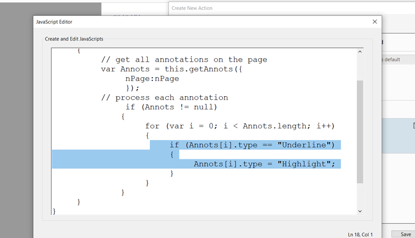
Uncheck the ‘Prompt User’ box, and then add the Save step to the action, so you will not be prompted to save each file when the action runs.
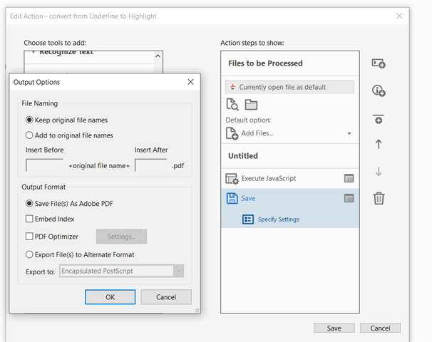
After saving and running the action, you can process multiple files by selecting the options in the drop down menu to add files or an entire folder.
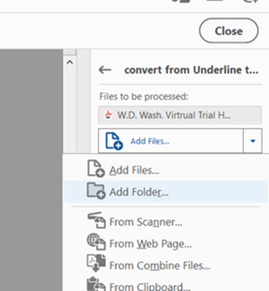
The script can be used to convert multiple proposed redactions in multiple PDF files like this:
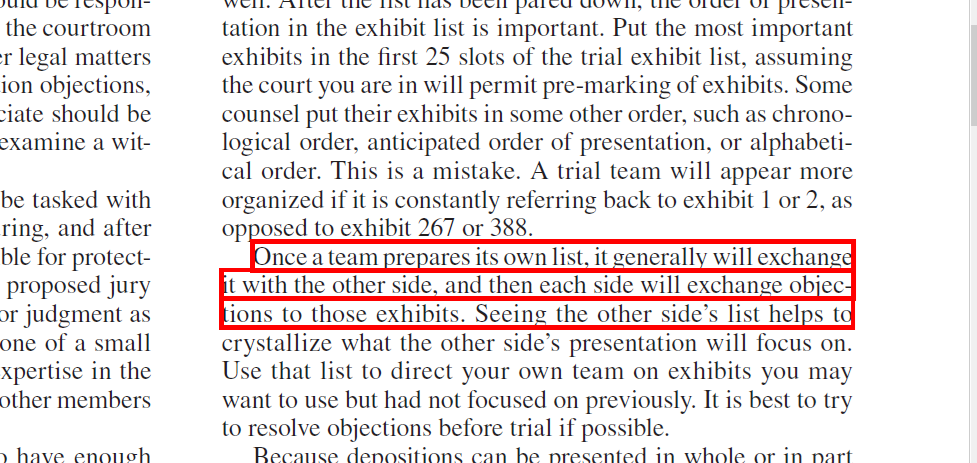
The script will convert one or more lines of continuous text selected for a redaction, but it will not convert a large block of text set for redaction.
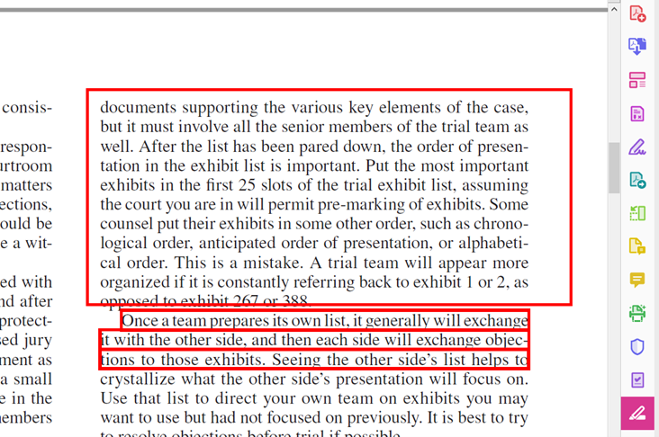
The action will give this result:
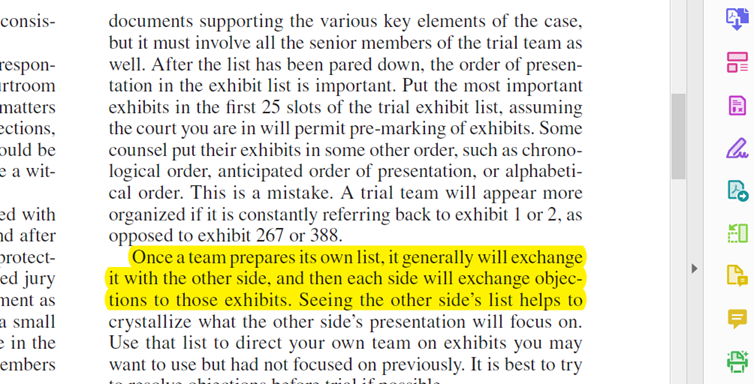
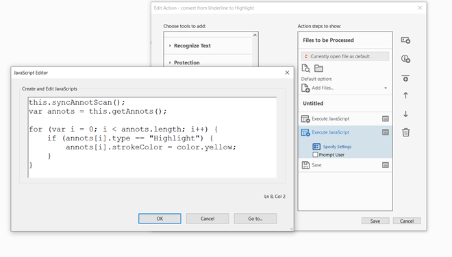
You can add a second javascript to the same action to specify the highlighting color you want the action to convert annotations or proposed redactions to:
this.syncAnnotScan();
var annots = this.getAnnots();
for (var i = 0; i < annots.length; i++) {
if (annots[i].type == “Highlight”) {
annots[i].strokeColor = color.yellow;
}
}
try
{
this.syncAnnotScan();
for (var nPage = 0; nPage < this.numPages; nPage++)
{
// get all annotations on the page
var Annots = this.getAnnots({
nPage:nPage
});
// process each annotation
if (Annots != null)
{
for (var i = 0; i < Annots.length; i++)
{
if (Annots[i].type == “StrikeOut”)
{
Annots[i].type = “Highlight”;
}
}
}
}
}
catch(e)
{
app.alert(e);
}

